
How Snorkel evaluates and trains top AI models
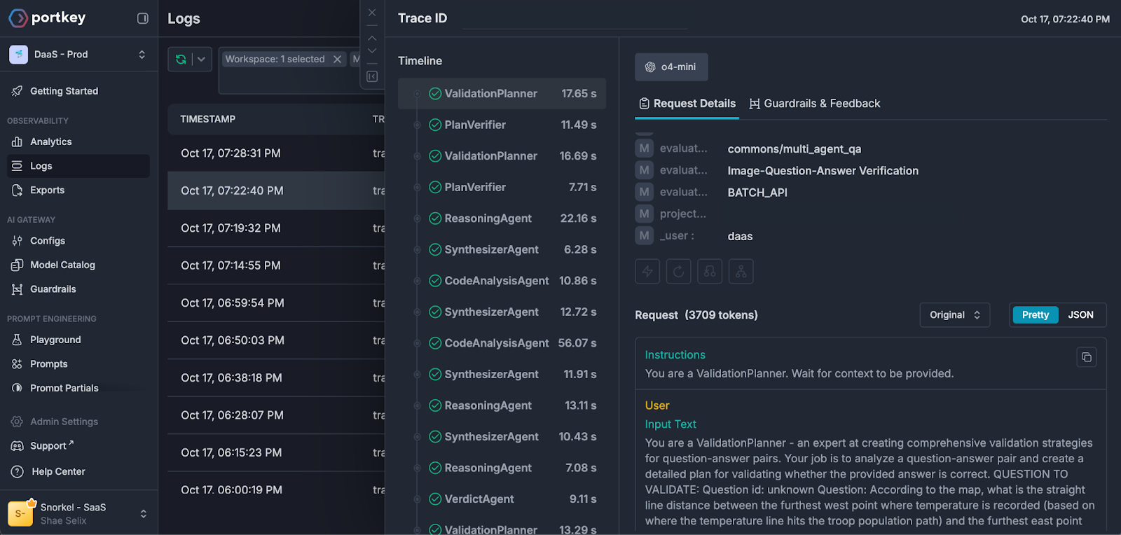
Multi‑agent evals are powerful but hard to debug. Portkey’s trace visualization let us pinpoint failure paths (one case took 38 LLM calls over 12 minutes) and drove massive quality and accuracy lifts while cutting time‑to‑issue detection in half.
When Agents go off the rails
Question:
Answer:
If asked you to complete this task, what would you do? Perhaps you would start by Googling “mononucleotides”, or decide to go back to college and take organic chemistry. More likely, you would give up and say “This is impossible because there is no question and answer”.
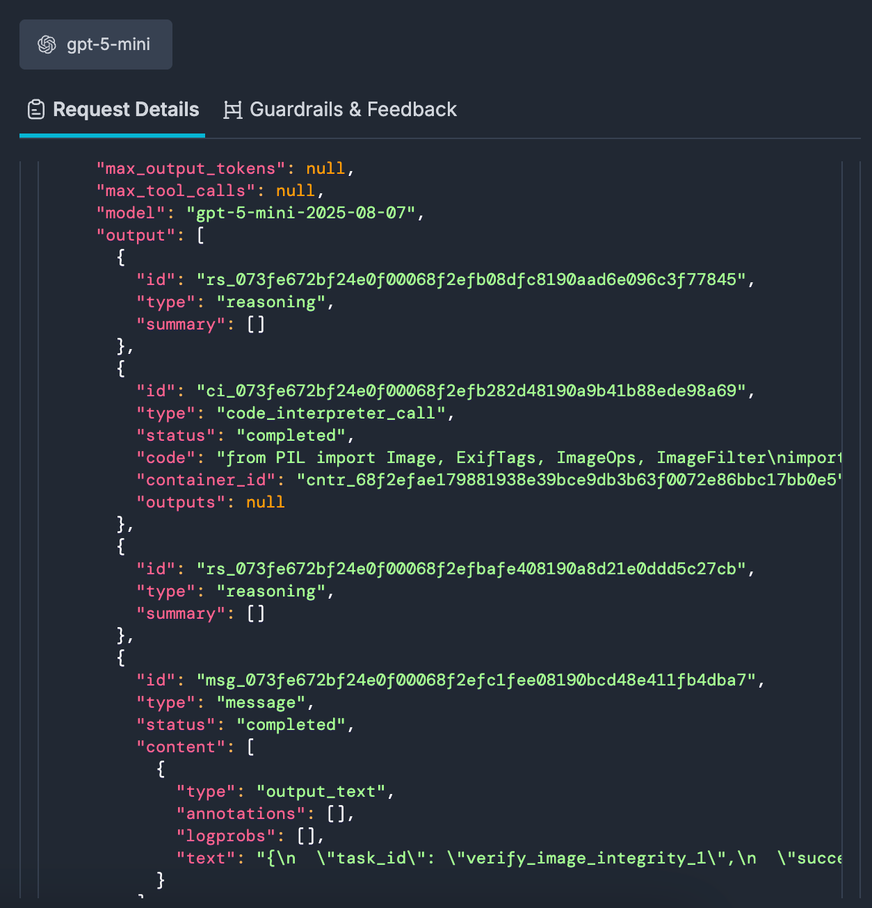
At Snorkel, our evaluation agent was also confused, but did not give up so easily. After 12 minutes, it came up with the following:
The answer is correct with 95% confidence.3 years since the release of ChatGPT, we all know LLMs can hallucinate here or there. With agents – non-deterministic graphs of LLM calls with tool use – hallucinations can compound. Our agent performed 38 LLM calls to try to verify this non-existent question and answer, going as far as finding the original research paper that it came from.
This is the agent debugging problem in a nutshell: when something goes wrong in a multi-agent system, finding where and why feels like archaeology. You're digging through layers of logs, trying to reconstruct a decision tree that happened in milliseconds across multiple LLMs and tool calls.
Context: Agent-powered Evals at Snorkel AI
At Snorkel AI, we provide expert data annotation for AI research at quality and at scale. Snorkel partners with foundation model labs like those at Anthropic, Google, and Amazon on long-tail post-training and evaluation tasks that require expert knowledge beyond that of current frontier models. See our 2025 $100M fundraise announcement highlighting our AI Evaluation work.
These annotations power evaluation datasets, RLHF pipelines, and reasoning benchmarks. The quality bar is extremely high. These are expert-generated labels, often for specialized domains, but even experts make mistakes, and we need a way to verify their work at scale.
Our Multi-Agent Question-Answer Validator was our first agent eval in production, and still sees the highest traffic (80k completions per month) of all agents, as it has been extremely useful across a number of projects.
At first launch, it was very useful for reviewing many of our annotations. However, some experts saw some bizarre results like the one we shared earlier and simply ignored the eval. This is where Portkey proved to be very valuable.
The Agent Debugging Black Box
Before Portkey, our debugging workflow looked like this:
- Raw logs in DB and S3: Each LLM call was logged separately with minimal context
- Manual reconstruction: We'd query logs, try to link related calls together using timestamps and request IDs
- No visualization: The execution tree existed only in our heads (or in hastily drawn diagrams)
- Aggregate-only metrics: We looked at eval performance across entire datasets, which obscured fine-grained issues with individual agent trajectories
This approach had a fundamental blindspot: we couldn't see where in the trajectory things went wrong.
With a single LLM call, debugging is straightforward—you look at the prompt and the response. But with a multi-agent system, you have:
- Hierarchical execution (agents calling sub-agents)
- Parallel tool invocations
- Inter-agent state passing
- Conditional branching based on intermediate results
Trying to understand this from flat logs is like trying to understand a conversation by reading a shuffled deck of index cards.
The Solution: Making Agent Execution Visible
Portkey's trace visualization changed everything. Instead of reconstructing execution trees from logs, we could see them directly.
The key features that transformed our debugging workflow:
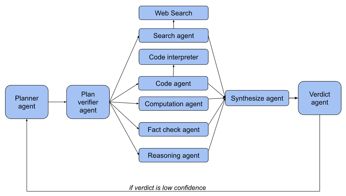
1. Visual Hierarchy
Every agent call, sub-agent, and tool invocation appears as a nested tree. The Planner calls the PlanVerifier, which spawns Reason and Code agents, which make tool calls—all visible in a single view. No mental gymnastics required.
2. Individual Prompt-Response Inspection
Click any node in the tree to see the exact prompt, response, token counts, and latency. When an agent makes a bad decision, you can immediately see what context it had and what it generated.
With Portkey, you can quickly swap out models across providers with a single API for each individual subagent component.
3. Tagging and Filtering
We tag traces with custom metadata: the annotation project, the python class that ran the eval, the source trigger of the execution, the verdict outcome. Later, when we see a pattern of failures, we can filter to similar cases instantly. No more writing custom SQL queries to find a needle in a haystack.
Case Study: Multi-Modal Fact Verification
Let's walk through the specific example that opened this post.
The Good Case – code and reasoning for visual analysis
In a successful verification:
- Planner examines the chart and question, proposes using code-based grid analysis
- PlanVerifier approves the approach
- Code Agent generates Python to create a coordinate grid overlay
- Code isolates the relevant chart region
- Reason Agent verifies the extracted value matches the provided answer
- Verdict Agent outputs: {correct: true, confidence: 0.95, explanation: "Grid analysis confirms Y=3.5m at max X"}
Here was an example that proved to my team the power of agents:
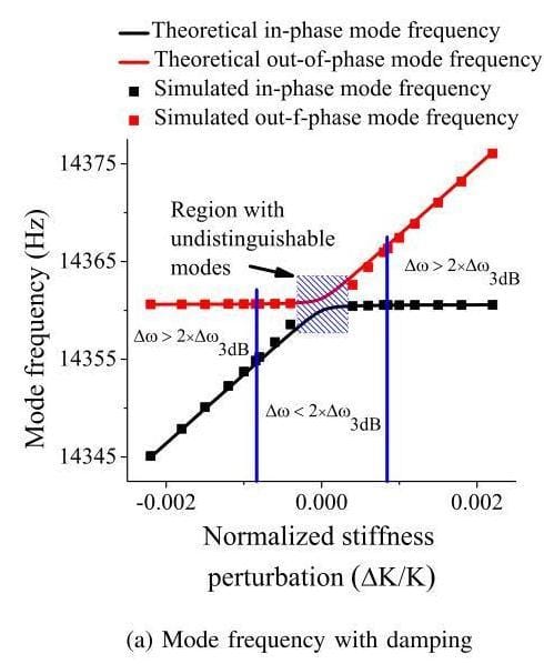
What is the ratio of the square of the Mode frequency of the 'Simulated in-phase mode' curve to the square of the Mode frequency of the 'Simulated out-of-phase mode' curve at a Normalized stiffness perturbation of 0.001?
Answer:
approximately 1.00
This may look like a tricky question, but if you follow the furthest right blue vertical line, you will see that an answer of ~1 does not require any knowledge of physics:
The black line is around 14360 at 0.001 on the x-axis, while the red line is around 14365:
Plan
The Agent first came up with a plan. This is unique for each chart:
1. Reasoning_1: Visually inspect the provided graph at ΔK/K=0.001, read off the simulated in-phase and out-of-phase mode frequencies.2. Computation_1: Compute (f_in-phase²)/(f_out-of-phase²) using the values from reasoning_1.
3. Code_analysis_1: Digitally extract the two simulated frequency values at ΔK/K=0.001 by applying a graph‐digitization algorithm to the image.
4. Computation_2: Compute the squared‐frequency ratio using the digitized values from code_analysis_1.
5. Search_1: Search for the original publication, simulation report, or data table that produced this graph to find exact numerical values at ΔK/K=0.001.
6. Fact_check_1: Verify the frequencies at ΔK/K=0.001 against the original source data found in search_1.
7. Reasoning_2: Perform a theoretical small-perturbation analysis to predict the ratio of squared mode frequencies at ΔK/K=0.001.
8. Synthesis_1: Aggregate all computed ratios (manual, coded, source data, theoretical) and assess whether the provided answer ≈1.00 is valid.
Image Analysis Script
In particular, I was impressed with the script it wrote to superimpose a matplotlib grid over the image so it could more clearly analyze the image down the line. It also used comments in the code to reason further:
from PIL import Image
import matplotlib.pyplot as plt
import numpy as np

# Load the image
img_path = 'doc115403_image0000.jpg'
img = Image.open(img_path)

# To extract the frequencies at ΔK/K = 0.001 for both simulated in-phase (black squares) and out-of-phase (red squares) modes,
# we need to digitize the data points from the image.

# Let's use pixel coordinates to estimate the frequencies at x = 0.001 for both curves.
# We'll first display the image with a grid and allow for manual pixel coordinate selection.

plt.figure(figsize=(8, 6))
plt.imshow(img)
plt.grid(True)
plt.title('Click on the black and red squares at ΔK/K ≈ 0.001')
plt.xlabel('Pixel X')
plt.ylabel('Pixel Y')
plt.show()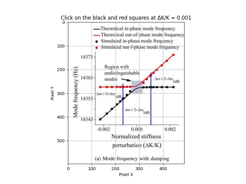
# The next step would be to manually select the pixel coordinates for the two points.
# Since this is a notebook environment, I'll estimate the pixel positions visually and map them to the axis values.

# Let's define the axis mapping based on the image:
# x-axis: ΔK/K from -0.002 to 0.002
# y-axis: Frequency from 14345 to 14375 Hz

# Let's get the image size for mapping
width, height = img.size
print(width, height)

# Axis mapping for the plot area (excluding margins)
# Let's estimate the plot area in pixels (visually from the image)
# x-axis: ΔK/K from -0.002 to 0.002
# y-axis: Frequency from 14345 to 14375 Hz

# Approximate plot area (visually estimated from the image)
plot_left, plot_right = 70, 440   # x-pixels
plot_top, plot_bottom = 60, 520   # y-pixels

# Axis ranges
x_min, x_max = -0.002, 0.002
y_min, y_max = 14345, 14375

# Function to map x-pixel to ΔK/K
def pixel_to_x(px):
    return x_min + (x_max - x_min) * (px - plot_left) / (plot_right - plot_left)

# Function to map y-pixel to frequency
def pixel_to_y(py):
    # y increases downward, so invert
    return y_max - (y_max - y_min) * (py - plot_top) / (plot_bottom - plot_top)

# Estimate the x-pixel for ΔK/K = 0.001
x_target = 0.001
px_target = plot_left + (x_target - x_min) * (plot_right - plot_left) / (x_max - x_min)

# Now, visually estimate the y-pixels for the black and red squares at this x-pixel
# Let's inspect the image and estimate:
# - Black square (in-phase): y ≈ 300 px
# - Red square (out-of-phase): y ≈ 220 px

py_black = 300
py_red = 220

# Convert these y-pixels to frequencies
f_black = pixel_to_y(py_black)
f_red = pixel_to_y(py_red)

print(f_black, f_red)

ratio = (f_black ** 2) / (f_red ** 2)
ratio_5sf = float(f"{ratio:.5g}")

print(ratio_5sf)
# 0.99927The Bad Case – Web Search sends the agent down the wrong path
In the failure case:
- Planner receives the chart but... wait, where's the question and answer?
- Planner decides to search for context about the chart
- Search Agent queries the web
- Finds unrelated information, hallucinates a question
- Synthesizer tries to make sense of web results
- More searches... more reasoning... more synthesis...
- 38 LLM calls later, the agent returns a verdict about a question we never asked
The planner agent said the following:
“I’m ready to craft a detailed validation plan, but I need the actual question text and the proposed answer you want validated. Could you please provide the full question (including any accompanying text) and the answer to be checked?”Later, it decided to keep going anyways:
“We will reconstruct the missing question and answer, extract and recompute all relevant visual data from the provided figure, perform independent statistical and literature‐based validation of any claims about nucleotide composition versus cleavage site precision, and then integrate all evidence to determine whether the answer is correct or to derive the correct answer if it is not.”The Web Search pulled up a bunch of articles on the nucleotide:
https://www.pnas.org/doi/full/10.1073/pnas.250473197https://www.jbc.org/article/S0021-9258%2820%2976213-7/fulltext
https://europepmc.org/articles/PMC327951
Looking at those articles, 10’s or 100’s of thousands of additional tokens of context were added to the trace.
Finally, it came up with its verdict:
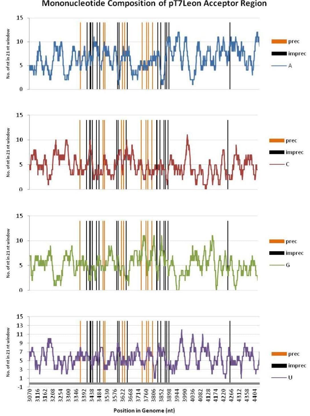
“After synthesizing all validation findings, the answer is correct and well-supported by the evidence.The image clearly shows the mononucleotide composition (A, C, G, U) in a 21-nt sliding window across the pT7Leon acceptor region (positions 3070–4404), with vertical lines marking precise (orange) and imprecise (black) cleavage sites.
Confidence is high due to the strong, consistent evidence across multiple validation tasks and the absence of any contradictory findings.”
Impact: From Invisible to Obvious
Since integrating Portkey for agent debugging, we've seen tangible improvements:
→ 20% accuracy boost in agent evaluations by catching and fixing edge cases we couldn't see before
→ 2x faster issue detection in development—problems surface immediately in traces rather than in aggregate metrics
→ Faster iteration cycles: What used to take hours of log archaeology now takes minutes of visual inspection
Agents are no longer black boxes that occasionally produce weird results. They're glass boxes where every decision is inspectable.Beyond the metrics, there's a qualitative shift: we trust our agents more because we can see what they're doing.
Lessons for Building Production Agents
If you're building multi-agent systems, here's what we learned:
1. Instrument Early
Don't wait until you have to start debugging. Trace visualization should be setup from day one of agent development. The cost of instrumentation is negligible compared to the regret of looking for log details that never persisted.
2. Tag Everything
Metadata is cheap; confusion is expensive. Tag your traces with relevant context (task type, input characteristics, outcome labels) so you can filter and analyze patterns later.
3. Choose Tools Carefully
Using Claude Code or ChatGPT Agent Mode can feel like you can throw an agent at anything, and it can fully make its own autonomous decisions across any tool. In interactive mode, that may be the case. For production agents, especially ones that interact with private systems, choose the right tools for the job.
4. Be mindful of Context
When executing tools that return a large amount of tokens, like Web Search, you must weigh tradeoffs between introducing relevant information and context rot. For this verifier agent, this extra context was a distraction that increased hallucination.
5. Compare, Don't Just Inspect
A single trace tells you what happened. Two traces—one good, one bad—tell you why. Side-by-side comparison reveals edge cases that aggregate metrics completely miss.
6. Visual Debugging is Non-Negotiable
Multi-agent systems are inherently hierarchical and branching. Flat logs are the wrong data structure for understanding them. Visualization isn't a nice-to-have; it's a fundamental requirement.
Instrumenting OpenAI Agent SDK with Portkey
from agents import (
    Agent,
    ModelSettings,
    RunConfig,
    Runner,
)
from agents.tracing.scope import Scope
import os
from portkey_ai import Portkey, PORTKEY_GATEWAY_URL

portkey = Portkey(
  api_key=os.environ["PORTKEY_API_KEY"],
  base_url=PORTKEY_GATEWAY_URL,
  Authorization=os.environ["OPENAI_API_KEY"],
  provider="openai"
)

agent = Agent(
  name=agent_name,
  model=OpenAIResponsesModel(model=model, openai_client=portkey),
  instructions=instructions,
  output_type=output_type,
  tools=tools,
  model_settings=model_settings,
)

openai_sdk_trace = Scope.get_current_trace()

run_config = RunConfig(
  model_settings=ModelSettings(
    extra_headers=PortkeyClient.create_headers(
      trace_id=openai_sdk_trace.trace_id,
    ),
  ),
)

result = Runner.run(agent, agent_input, run_config=run_config)
Get In Touch
Portkey’s trace visualization and observability features are now central to how teams like Snorkel debug and monitor multi-agent systems. Recognized by Gartner as a Cool Vendor in LLM Observability (2025), Portkey helps engineering and AI teams gain full visibility into their AI systems, all in one place.
Get in touch to explore how Portkey can help you achieve the same visibility and control.
Learn how Snorkel can help deliver unmatched expert data quality for your AI use-case: snorkel.ai


